Introduction
In this talk/document/presentation I showcase some of the possibilities that a combination of tools provides:
In order to make sure things look good from the first start, you might check out some additional projects and files:
- Bootstrap template for Pandoc: https://github.com/tonyblundell/pandoc-bootstrap-template
- Alternative LaTeX templates: https://github.com/kjhealy/latex-custom-kjh
- Alternative Pandoc template: https://github.com/kjhealy/pandoc-templates
- Non-official KU Leuven templates: https://github.com/exporl/kuleuven-templates
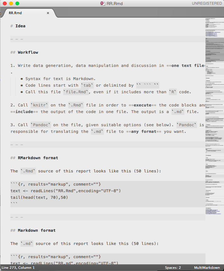
Idea
Workflow
- Write data generation, data manipulation and discussion in one text file.
- Syntax for text is Markdown.
- Code lines start with
tabor delimited by``` - Call this file
file.Rmd, even if it includes more thanRcode.
Call
knitron the.Rmdfile in order to execute the code blocks and include the output of the code in one file. The output is a.mdfile.Call
Pandocon the file, given suitable options (see below).Pandocis responsible for translating the.mdfile to any format you want.
RMarkdown format
The .Rmd source of this report looks like this (50 lines):
text <- readLines("RR.Rmd",encoding="UTF-8")
tail(head(text, 70),50)
[1] " <https://github.com/tonyblundell/pandoc-bootstrap-template>"
[2] "* Alternative LaTeX templates: "
[3] " <https://github.com/kjhealy/latex-custom-kjh>"
[4] "* Alternative Pandoc template: "
[5] " <https://github.com/kjhealy/pandoc-templates>"
[6] "* Non-official KU Leuven templates:"
[7] " <https://github.com/exporl/kuleuven-templates>"
[8] ""
[10] ""
[11] "# Idea"
[12] ""
[14] ""
[15] "## Workflow"
[16] ""
[17] "1. Write data generation, data manipulation and discussion in **one text file**."
[18] " * Syntax for text is Markdown."
[19] " * Code lines start with `tab` or delimited by `` ``` ``"
[20] " * Call this file `file.Rmd`, even if it includes more than `R` code."
[21] ""
[22] "2. Call `knitr` on the `.Rmd` file in order to **execute** the code blocks and **include** the output of the code in one file. The output is a `.md` file."
[23] ""
[24] "3. Call `Pandoc` on the file, given suitable options (see below). `Pandoc` is responsible for translating the `.md` file to **any format** you want. "
[25] ""
[27] ""
[28] "## RMarkdown format"
[29] ""
[30] "The `.Rmd` source of this report looks like this (50 lines):"
[31] ""
[32] "```{r, results=\"markup\", comment=\"\"}"
[33] "text <- readLines(\"RR.Rmd\",encoding=\"UTF-8\")"
[34] "tail(head(text, 70),50)"
[35] "```"
[36] ""
[38] ""
[39] "## Markdown format"
[40] ""
[41] "The `.md` source of this report looks like this (50 lines):"
[42] ""
[43] "```{r, results=\"markup\", comment=\"\"}"
[44] "text <- readLines(\"RR.md\",encoding=\"UTF-8\")"
[45] "tail(head(text, 70),50)"
[46] "```"
[47] ""
[48] "Conversion is done using `knitr`."
[49] "" Markdown format
The .md source of this report looks like this (50 lines):
text <- readLines("RR.md",encoding="UTF-8")
tail(head(text, 70),50)
[1] " <https://github.com/tonyblundell/pandoc-bootstrap-template>"
[2] "* Alternative LaTeX templates: "
[3] " <https://github.com/kjhealy/latex-custom-kjh>"
[4] "* Alternative Pandoc template: "
[5] " <https://github.com/kjhealy/pandoc-templates>"
[6] "* Non-official KU Leuven templates:"
[7] " <https://github.com/exporl/kuleuven-templates>"
[8] ""
[10] ""
[11] "# Idea"
[12] ""
[14] ""
[15] "## Workflow"
[16] ""
[17] "1. Write data generation, data manipulation and discussion in **one text file**."
[18] " * Syntax for text is Markdown."
[19] " * Code lines start with `tab` or delimited by `` ``` ``"
[20] " * Call this file `file.Rmd`, even if it includes more than `R` code."
[21] ""
[22] "2. Call `knitr` on the `.Rmd` file in order to **execute** the code blocks and **include** the output of the code in one file. The output is a `.md` file."
[23] ""
[24] "3. Call `Pandoc` on the file, given suitable options (see below). `Pandoc` is responsible for translating the `.md` file to **any format** you want. "
[25] ""
[27] ""
[28] "## RMarkdown format"
[29] ""
[30] "The `.Rmd` source of this report looks like this (50 lines):"
[31] ""
[32] ""
[33] "```r"
[34] "text <- readLines(\"RR.Rmd\",encoding=\"UTF-8\")"
[35] "tail(head(text, 70),50)"
[36] "```"
[37] ""
[38] "```"
[39] " [1] \" <https://github.com/tonyblundell/pandoc-bootstrap-template>\" "
[40] " [2] \"* Alternative LaTeX templates: \" "
[41] " [3] \" <https://github.com/kjhealy/latex-custom-kjh>\" "
[42] " [4] \"* Alternative Pandoc template: \" "
[43] " [5] \" <https://github.com/kjhealy/pandoc-templates>\" "
[44] " [6] \"* Non-official KU Leuven templates:\" "
[45] " [7] \" <https://github.com/exporl/kuleuven-templates>\" "
[46] " [8] \"\" "
[48] "[10] \"\" "
[49] "[11] \"# Idea\" "
[50] "[12] \"\" "Conversion is done using knitr.
Pandoc
A simple and a more involved example of running Pandoc:
pandoc file.md -o file.docx

pandoc file.md -o file.html \
      -t html5 \
            --template template.html \
            --css template.css \
            --highlight-style=tango --mathjax \
            --toc --toc-depth 2
Dust off your Makefile skills!
Some Examples
Simple example
The first example is in R. Let's say I want to plot a function
\[ f(x) = \frac{\log(x^2+x+1)}{2x} \]
We first define \(x\) and the function value \(y\) (in doing so we have used some inline equations as well):
x <- seq(from=-5,to=10,by=.01)
y <- (log(x*x + x + 1))/(2*x)
Then we can plot the function. We use the ggplot2 package.
library(ggplot2)
qplot(x,y,geom="line")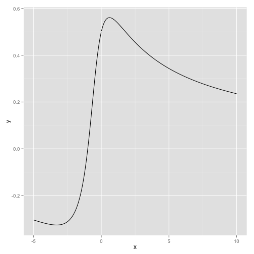
See the figure for the result.
Working with data
Let us take a look at a dataset that comes with R, mtcars:
summary(mtcars)## mpg cyl disp hp
## Min. :10.40 Min. :4.000 Min. : 71.1 Min. : 52.0
## 1st Qu.:15.43 1st Qu.:4.000 1st Qu.:120.8 1st Qu.: 96.5
## Median :19.20 Median :6.000 Median :196.3 Median :123.0
## Mean :20.09 Mean :6.188 Mean :230.7 Mean :146.7
## 3rd Qu.:22.80 3rd Qu.:8.000 3rd Qu.:326.0 3rd Qu.:180.0
## Max. :33.90 Max. :8.000 Max. :472.0 Max. :335.0
## drat wt qsec vs
## Min. :2.760 Min. :1.513 Min. :14.50 Min. :0.0000
## 1st Qu.:3.080 1st Qu.:2.581 1st Qu.:16.89 1st Qu.:0.0000
## Median :3.695 Median :3.325 Median :17.71 Median :0.0000
## Mean :3.597 Mean :3.217 Mean :17.85 Mean :0.4375
## 3rd Qu.:3.920 3rd Qu.:3.610 3rd Qu.:18.90 3rd Qu.:1.0000
## Max. :4.930 Max. :5.424 Max. :22.90 Max. :1.0000
## am gear carb
## Min. :0.0000 Min. :3.000 Min. :1.000
## 1st Qu.:0.0000 1st Qu.:3.000 1st Qu.:2.000
## Median :0.0000 Median :4.000 Median :2.000
## Mean :0.4062 Mean :3.688 Mean :2.812
## 3rd Qu.:1.0000 3rd Qu.:4.000 3rd Qu.:4.000
## Max. :1.0000 Max. :5.000 Max. :8.000Now the fun starts. Let's fit a model relates how many Miles/Gallon are consumed, given a weight.
model <- lm(mpg ~ wt, data=mtcars)
summary(model)
##
## Call:
## lm(formula = mpg ~ wt, data = mtcars)
##
## Residuals:
## Min 1Q Median 3Q Max
## -4.5432 -2.3647 -0.1252 1.4096 6.8727
##
## Coefficients:
## Estimate Std. Error t value Pr(>|t|)
## (Intercept) 37.2851 1.8776 19.858 < 2e-16 ***
## wt -5.3445 0.5591 -9.559 1.29e-10 ***
## ---
## Signif. codes: 0 '***' 0.001 '**' 0.01 '*' 0.05 '.' 0.1 ' ' 1
##
## Residual standard error: 3.046 on 30 degrees of freedom
## Multiple R-squared: 0.7528, Adjusted R-squared: 0.7446
## F-statistic: 91.38 on 1 and 30 DF, p-value: 1.294e-10This is verbatim output, we can use some R package magic to get proper tables as output as well using the pander package:
library(pander)
pander(model)| Estimate | Std. Error | t value | Pr(>|t|) | |
|---|---|---|---|---|
| wt | -5.344 | 0.5591 | -9.559 | 1.294e-10 |
| (Intercept) | 37.29 | 1.878 | 19.86 | 8.242e-19 |
We can also plot this information using the code below.
qplot(x=wt, y=mpg, data=mtcars, xlab="Weight (lb/1000)", ylab="Miles per Gallon",
      geom=c("point","smooth"), method="lm")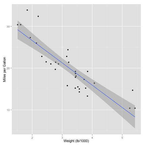
Scraping the web
This script parses the Wikipedia page with Belgian Beers in order to get the data out. It then does some cleaning up and converts the data to different formats. The result can be stored in a file, but just display the first 10 rows.
library(XML)
rawBeers <- readHTMLTable(doc="http://nl.wikipedia.org/wiki/Lijst_van_Belgische_bieren")
beers <- NULL

# The first table is not relevant, the rest is:
for (i in seq(2,28)) {
  beers <- rbind(beers,rawBeers[[i]])
}

# Remove the percentage sign and convert to numbers:
beers$Percentagealcohol <- gsub("%","",beers$Percentagealcohol)
beers$Percentagealcohol <- gsub(",",".",beers$Percentagealcohol)
beers$Percentagealcohol <-as.numeric(beers$Percentagealcohol)
## Warning: NAs introduced by coercion# A few entries do not have a percentage entry
nas <- length(beers[is.na(beers$Percentagealcohol),])The number of entries without percentage entry is: 4.
We use pander again for displaying the top-10 of beers with the highest amount of alcohol:
pander(
  head(
    beers[order(beers$Percentagealcohol,decreasing=TRUE),
          c("Merk","Percentagealcohol")],
    10)
)| Merk | Percentagealcohol | |
|---|---|---|
| 196 | Black Damnation V (Double Black) | 26 |
| 412 | Cuvée d'Erpigny | 15 |
| 191 | Black Albert | 13 |
| 192 | Black Damnation I | 13 |
| 194 | Black Damnation III (Black Mes) | 13 |
| 195 | Black Damnation IV (Coffée Club) | 13 |
| 313 | Bush de Noël Premium | 13 |
| 314 | Bush de Nuits | 13 |
| 315 | Bush Prestige | 13 |
| 411 | Cuvée Delphine | 13 |
Different languages
Python
import pprint
pprint.pprint(zip(('Byte', 'KByte', 'MByte', 'GByte', 'TByte'),
              (1 << 10*i for i in xrange(5))))
## [('Byte', 1),
## ('KByte', 1024),
## ('MByte', 1048576),
## ('GByte', 1073741824),
## ('TByte', 1099511627776)]Scala
val collection = for {i <- 1 to 10} yield {i}
val mapped = collection map (x => x*x)
val reduced = mapped reduce (_ + _)
println(reduced)
## 385Sweave
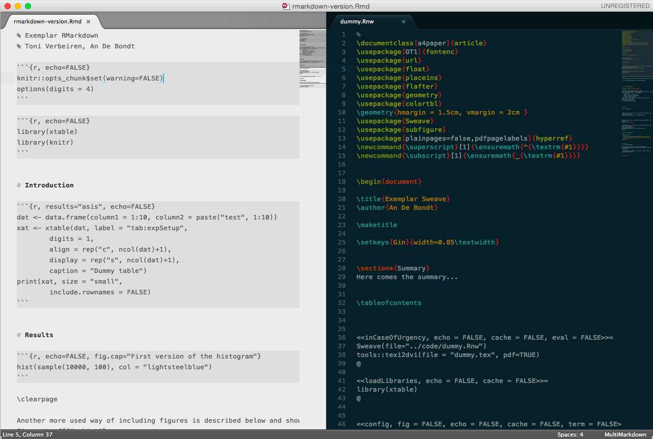
knitr can handle sweave documents as well.
library(knitr)
Sweave2knitr('dummy.Rnw')
knit('dummy-knitr.Rnw')
Or, just write in RMarkdown:
Rscript -e 'library(knitr); knit("rmarkdown-version.Rmd")
pandoc rmarkdown-version.md -o rmarkdown-version.pdf --toc
Text (and code) can be translated using Pandoc
What to use it for?
I use it for:
- Creating presentations (
reveal.js) - Writing reports (including code)
- Writing papers (just text)
- Making coffee
How to use it?
RStudio
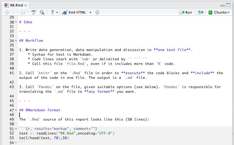
your favourite editor here
Additional pointers
- Markdown to
Reveal.js: http://tverbeiren.github.io/BigDataBe-Spark/#/ - Markdown and
Pandocfor writing a paper: http://homes.esat.kuleuven.be/~bioiuser/blog/?p=243 - Markdown and
Pandocfor lecture notes: https://bitbucket.org/tverbeiren/i0u19a - You can find everything I showed here at: http://github.io/tverbeiren/ReproducibleDataAnalysis/